
Author's posts
Sep 06
How to Create a “Chainsaw” List of Excel Worksheet Functions
By David Ringstrom, CPA
Depending upon your version of Excel, you have nearly 500 different worksheet functions at your disposal. Some worksheets functions, such as CUMIPMT and NPER, are like the chainsaw in my garage. I don’t use them very often, but when I do, no other tool will suffice. Other functions are more akin to screwdrivers and pliers in that I use these so often that I can type them in my sleep. In this article I’ll show you an easy way to keep a “chainsaw” list of functions at the ready, so you can avoid trying to remember “how’d I do that before?”
We’ll store our list in an unlikely location known as the Name Box. It’s pretty much impossible to use Excel and not notice the Name Box, which appears just above the upper-left-hand corner of the worksheet frame. Most users know this as the space in Excel where you can determine the address of the currently selected cell.
Continue reading on www.accountingweb.com
David H. Ringstrom, CPA heads up Accounting Advisors, Inc., an Atlanta-based software and database consulting firm providing training and consulting services nationwide. Contact David at david@acctadv.com or follow him on Twitter. David speaks at conferences about Microsoft Excel, and presents webcasts for several CPE providers, including AccountingWEB partner CPE Link
Aug 31
Build a Dynamic Income Tax Calculator – Part 2 of 2
By David H. Ringstrom, CPA
(If you didn’t already do so in Part 1, click here to download the accompanying Income Tax Calculator spreadsheet.)
Last month I explained how to use the VLOOKUP function to cross-reference tax rates from a tax rate table. I then extended the functionality by creating 4 different tables — Single, Married-Joint, Married-Single, and Head of Household, as shown in Figure 1. After assigning a range name to each table, I used Microsoft Office Excel’s Data Validation feature to create an in-cell drop-down list comprised of these range names. Finally, I modified my VLOOKUP functions to use Excel’s INDIRECT function. INDIRECT replaced the static look-up range originally specified in the VLOOKUP formula. If I choose Married-Joint from the list, the VLOOKUP function will calculate the tax due based on that table. I can choose Married-Single from the list to determine the additional tax due under that filing status. At this point I have an efficient calculator for determining the amount due based on a taxable income input, but I’d rather not have 4 separate tables. This month I’ll dig deeper, and show you how to create a single table of tax rates, as shown in Figure 2. The final result will involve two rather complex formulas, but we’ll build them a step at a time.
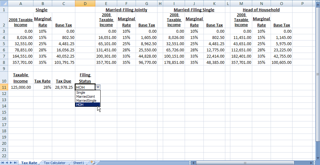 Figure 1: The VLOOKUP version of the tax calculator relies on four separate rate tables.
 Figure 2: The new tax calculator will rely on a single rate table.
Understand MATCH
The MATCH function is akin to VLOOKUP — you specify what to look for, where to look, and the type of match that you’d like. When the MATCH function finds the criteria you specify, it returns the position number within the list —otherwise it returns #N/A. The position number can then be used within an INDEX function to return a specific value, much like VLOOKUP or HLOOKUP. Although VLOOKUP is a useful look-up function, your look-up criteria must always be the first column of your data table. Instead, the INDEX/MATCH combination enables you to create a look-up based on any column within the table.
The MATCH function has three arguments:
- Look-up value: What we’re looking for, such as a taxable income amount.
- Look-up array: A single column range that contains the potential look-up values, such as the taxable income tiers associated with various income tax rates.
- Match type: We can choose from three different match types:
- -1 instructs MATCH to find the smallest value that is greater than or equal to the look-up value. In this case the list must be sorted in descending order.
- 0 instructs MATCH to find an exact match. In this case the list can be in any order.
- 1 instructs MATCH to find the largest value that is less than or equal to the look-up value. In this case the table must be sorted in ascending order.
Since MATCH only returns the position number within the list, we’ll then use the INDEX function to return actual amounts from the table.
Comprehend INDEX
I only have space in this article to describe the reference capability of the INDEX function, but Excel’s Help feature discusses the array and multiple area capabilities of INDEX. The reference capability of INDEX has three arguments:
- Reference: Typically this is the address of a table, such cells B2:J8 in Figure 2.
- Row number: This argument tells the INDEX function to look at a specified row within the table. In the case of our tax calculator, we’ll use the MATCH function to provide this value.
- Column number: This optional argument provides the column coordinate. You can omit the column number if you provide a single-column range for the reference argument.
Appreciate OFFSET
Not many Excel users know about the OFFSET function. In essence, it’s a means for shifting a range a certain number of columns and/or rows away from a starting point. In the case of our tax calculator, we’ll use OFFSET to have the MATCH function refer to the proper columns within our tax rate table. The OFFSET function has five arguments:
- Reference: The starting point for our range, such as A2:A8.
- Rows: The number of rows away from the starting point that you’d like the range to be shifted. Use a negative number to shift the range upward, or a positive number to move it down. Specify zero if you do not want to shift the range from the starting point. We’ll use zero, because we won’t want to shift the rows.
- Columns: The number of columns away from the starting point that you’d like the range to be shifted. Use a negative number to shift the range to the left, or a positive number to move it to the right. Specify zero if you do not want to shift the range from the starting point. We’ll use MATCH to shift the range to the right to correspond with the filing status that we choose from the drop-down list.
- Height: Indicates the height of the range in rows. Omit the argument if you don’t want to adjust the height of the range. We’ll omit this since we won’t need to adjust the height of our range.
- Width: Indicates the width of the range in columns. Omit this argument if you don’t want to adjust the width of the range. We’ll omit this since we won’t need to adjust the width of our range.
Create the Tax Calculator
Now that we have the function basics out of the way, let’s build a tax table that refers to a single table instead of four different tables. Enter these values in cells A2 through A8 of a blank worksheet:
|
Enter these values in cells B2 through C8 of the worksheet:
|
B2: |
Single |
C2: |
Base Tax |
|
B3: |
0.00 |
C3: |
0.00 |
|
B4: |
8,026.00 |
C4: |
802.50 |
|
B5: |
32,551.00 |
C5: |
4,481.25 |
|
B6: |
78,851.00 |
C6: |
16,056.25 |
|
B7: |
164,551.00 |
C7: |
40,052.25 |
|
B8: |
357,701.00 |
C8: |
103,791.75 |
Enter these values in cells D2 through E8 of the worksheet:
|
D2: |
Married-Joint |
E2: |
Base Tax |
|
D3: |
0.00 |
E3: |
0.00 |
|
D4: |
16,051.00 |
E4: |
802.50 |
|
D5: |
65,101.00 |
E5: |
4,481.25 |
|
D6: |
131,451.00 |
E6: |
16,056.25 |
|
D7: |
200,301.00 |
E7: |
40,052.25 |
|
D8: |
357,701.00 |
E8: |
103,791.75 |
Enter these values in cells F2 through G8 of the worksheet:
|
F2: |
Married-Single |
G2: |
Base Tax |
|
F3: |
0.00 |
G3: |
0.00 |
|
F4: |
8,026.00 |
G4: |
802.50 |
|
F5: |
32,551.00 |
G5: |
4,481.25 |
|
F6: |
65,726.00 |
G6: |
12,775.00 |
|
F7: |
100,151.00 |
G7: |
22,414.00 |
|
F8: |
178,851.00 |
G8: |
48,385.00 |
Enter these values in cells H2 through I8 of the worksheet:
|
H2: |
Head of Household |
I2: |
Base Tax |
|
H3: |
0.00 |
I3: |
0.00 |
|
H4: |
11,451.00 |
I4: |
1,145.00 |
|
H5: |
43,651.00 |
I5: |
5,975.00 |
|
H6: |
112,651.00 |
I6: |
23,225.00 |
|
H7: |
182,401.00 |
I7: |
42,755.00 |
|
H8: |
357,701.00 |
I8: |
100,605.00 |
Add these headings to the spreadsheet:
|
B10: |
Taxable Income |
|
C10: |
Tax Rate |
|
D10: |
Tax Due |
|
E10: |
Filing Status |
Enter 125,000 in cell B11, and then use Data Validation to create an in-cell drop-down list in cell E10:
- Excel 2007: Choose the Data Validation icon in the Data Tools section of the Data ribbon.
- Excel 2003 or earlier: Choose Tools, and then Data Validation.
- In all versions of Excel, choose List, and then enter this into the Source field, as shown in Figure 3:
Single,Married-Joint,Married-Single,Head Of Household
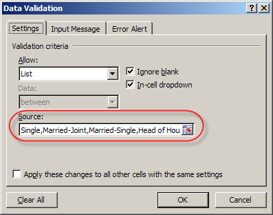
Figure 3: Enter the filing statuses in the Source field of the Data Validation window.
Caution: Be sure that the contents of the Source field exactly match the values that you entered in cells B2, D2, F2, and H2.
- Click OK. At this point, a drop-down list should appear when you click on cell E11, as shown in Figure 4. Choose Single from this list.
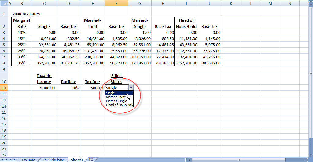 Figure 4: Data validation can provide an in-cell drop-down list.
We’ll now enter the formula to determine the tax rate. Enter this formula in cell C11:
=MATCH(B11,B3:B8,1)
Based on an input of 125,000 in cell B11, the formula should return the number 4. We’ve instructed MATCH to look at the taxable income for the Single filing status, and asked it to find the closest income bracket for $125,000. Next, we’ll add the INDEX function, so that we can get the actual tax rate. Modify the formula in cell C11 to be as follows:
=INDEX(A3:A8,MATCH(B11,B3:B8,1))
At this point the formula should return 28%. However, we’re referencing a static range of B3:B8 for our income brackets, and instead we want the formula to shift automatically based on our choice in cell E11. To do so, we’ll employ the OFFSET function. As shown in Figure 5, modify the formula in cell C11 to match this:
=INDEX(A3:A8,MATCH(B11,OFFSET(A3:A8,0,MATCH(E11,A2:I2,0)-1),1))
 Figure 5: This formula determines the tax rate based on the taxable income amount and filing status.
Although this may look intimidating, we basically replaced the B3:B8 portion of the formula with this component:
OFFSET(A3:A8,0,MATCH(E11,A2:I2,0)-1)
Our OFFSET function contains these arguments:
- Reference: A3:A8 serves as the starting point.
- Rows: Zero indicates that we don’t want to shift the range up or down.
- Columns: We use an additional MATCH function to determine which column in the table has our filing status. Notice that this time we used a zero for the match type, since we need an exact match. I subtracted 1, because in the case of Single, the MATCH function inside OFFSET returns 2, but I only need to shift over 1 column.
- Height: I omitted this argument, since I didn’t need to resize the range.
- Width: I omitted this argument, since I didn’t need to resize the range.
At this point the formula should return 28%. This number should change to 25% if you choose Married-Joint in cell E11, 33% for Married-Joint, or remain at 28% if you choose Head of Household.
We’re now ready to create the final formula in our table, which will perform the actual tax calculation. Enter this formula in cell D11:
=INDEX(A2:I8,MATCH(C11,A3:A8,0),MATCH(E11,A2:I2,0)+1)
In this case, we’re specifying the entire table range for the reference argument of the INDEX function, and then using two MATCH functions to return the row and column positions. This MATCH function determines the row for our tax rate:
MATCH(C11,A3:A8,0)
Notice the zero in the match type position, because we want to ensure an exact match on the tax rate. The second MATCH function determines which column has the base-tax amount:
MATCH(E11,A2:I2,0)+1
As before, we’re determining which column our filing status appears in within row 2, but then adding 1 to that amount, since the base tax amount is in the next column over.
We now need to calculate the marginal tax amount beyond the base tax. To do so, add this to the end of the formula in cell D11:
(B11-INDEX(A2:I8,MATCH(C11,A2:A8,0),MATCH(E11,A2:I2,0))+1)*C11
The INDEX function returns the tax tier associated with the tax rate, and this amount is subtracted from the taxable income. $1 is added to this amount to determine the precise marginal amount to be taxed, and then the amount in parenthesis is multiplied by the tax rate in cell C11. The complete formula is shown in Figure 6.
 Figure 6: The final piece of the calculator determines the tax due based on income level and filing status.
The views and opinions expressed in this column are those of the author and do not necessarily reflect the opinions of Microsoft.
This article first appeared Microsoft Professional Accountant’s Network newsletter.
David H. Ringstrom, CPA heads up Accounting Advisors, Inc., an Atlanta-based software and database consulting firm providing training and consulting services nationwide. Contact David at david@acctadv.com or follow him on Twitter. David speaks at conferences about Microsoft Excel, and presents webcasts for several CPE providers, including AccountingWEB partner CPE Link
Aug 31
Build a Dynamic Income Tax Calculator – Part 1 of 2
By David H. Ringstrom, CPA
Look-up formulas are one of Excel’s most powerful features. Instead of manually linking to a worksheet cell, such as =A2, a look-up formula allows you to provide a criteria, such as taxable income, and have the formula automatically return the proper tax rate. This enables you to quickly run through various scenarios with your clients by simply changing the taxable income value. However, income tax calculations in particular can become tricky, as your formula also needs to refer to one of four different tables. In part 1 of this two-part series I’ll explain how to use the VLOOKUP formula to cross-reference tax rates from a single table. I’ll then show you how to use Excel’s INDIRECT function make your VLOOKUP formula refer to the proper table based on your choice of filing status in an adjacent worksheet cell. Next month, in part 2 of this series, I’ll show you how to condense all four tables into one, and use the MATCH and INDEX functions instead of VLOOKUP.
Click here to download the accompanying Income Tax Calculator spreadsheet.
Understand VLOOKUP
As you might infer, VLOOKUP performs vertical look-ups, which means it looks at columnar ranges. A similar function, called HLOOKUP, looks across rows, but for this article I’ll only focus on VLOOKUP. This is an ideal function to use when you need a formula to return a marginal tax rate, as shown in Figure 1. First, let’s discuss the VLOOKUP function, which has 4 arguments:
- Lookup_Value: The value that you’re searching for within a table. For instance, this might be a contact’s name, a part number, or in Figure 1, an income tax rate.
- Table_Array: A range of two or more columns that comprises your data. For instance, in Figure 1, the tax brackets are in the first column, the marginal rate in the second column, and the base tax is in the third column. VLOOKUP always looks for the Lookup_Value in the first column of the table array.
- Col_Index_Num: The column number within the Table_Array contains the data that you want to return. Using Figure 1 as an example, we’d specify 2 if we want the income tax rate, or 3 for the base tax.
Caution: VLOOKUP will return a #VALUE! error if you enter a number less than 1 for the Col_Index_Num. Further, VLOOKUP will return a #REF! error if you specify a number greater than the number of columns in the Table_Array.
- Range_lookup: This optional argument enables you to specify between an approximate match or exact match:
- Approximate match: By default, VLOOKUP returns an approximate match, which means if it can’t find the Lookup_Value in the first column of the Table_Array then it returns the next largest value. You can either omit this argument, or enter TRUE to indicate that an approximate match is acceptable.
Trap: Approximate matches require the first column of the Table_Array be sorted in ascending order —otherwise VLOOKUP may return an incorrect value.
- Exact Match: Specify FALSE for this argument if only an exact match is acceptable. VLOOKUP returns #N/A if it cannot find the Lookup_Value in the first column of the Table_Array.
Caution: VLOOKUP matches on the first instance of the Lookup_Value. Thus, if your value appears more than once in column A, VLOOKUP will only return the first instance.
 Figure 1: We’ll use VLOOKUP to create a simple income tax calculator.
Marginal Tax Rate Look-Up
Now that you understand the inputs for VLOOKUP, let’s walk through an example:
- Enter the word Single into cell A1 of a blank worksheet.
- Enter these into cells A2 through C8 of a blank worksheet, as shown in Figure 1:
|
2008 Taxable Income |
Marginal Rate |
Base Tax |
|
0.00 |
10% |
0.00 |
|
8,026.00 |
15% |
802.50 |
|
32,551.00 |
25% |
4,481.25 |
|
78,851.00 |
28% |
16,056.25 |
|
164,551.00 |
33% |
40,052.25 |
- Enter the words Taxable Income in cell A10.
- Enter the words Tax Rate in cell B10.
- Enter a taxable income number in cell A11, such as 125,000.
- Enter this VLOOKUP formula cell B11:
=VLOOKUP(A11,A3:C8,2,TRUE)
The arguments for the function are as follows:
- A11 represents the Lookup_Value, which returns the taxable income amount
- A3:C8 represents the Table_Array, or the coordinates of the tax table
- 2 represents the Col_Index_Num, which indicates that we want the tax rate from the second column of the table
- True represents the Range_Lookup, which indicates that we want an approximate match, or the closest tax bracket for the taxable income amount.
The formula in cell B11 should return 28% if you entered 125,000 in cell A11.
Shortcut: Since we’re not seeking an exact match, we can omit the Range_Lookup argument and shorten the formula to this:
=VLOOKUP(A11,A3:C8,2)
Conversely, our formula would look like this if we did want an exact match:
=VLOOKUP(A11,A3:C8,2,FALSE)
Tax Calculation
Our formula in cell B11 now determines the marginal tax rate, so now we’ll calculate the tax liability. We can see that income of $125,000 places our taxpayer in the 28% tax bracket. However, 28% doesn’t apply to every dollar of their income — only to income greater than $78,850. We’ll add the base tax of $16,056.25 to this calculated amount, for a total tax of $28,978.25. The formula to perform this calculation is somewhat complex, so we’ll build it in stages:
- Enter the words Tax Liability in cell C10.
- Enter this formula in cell C11:
=VLOOKUP(A11,A3:C8,1)
We specify 1 for the Col_Index_Num, so that we can return the starting point of our tax bracket. Based on income of $125,000, the formula should return $78,851.
- Modify the formula in cell C11 to look like this:
=A10-(VLOOKUP(A11,A3:C8,1)-1)
Your formula should now return $46,150. In this case we’re taking our taxable income of $125,000 from cell A11, subtracting the tax bracket of $78,851, and then subtracting $1 from that amount. This is because our client must pay tax of 28% of all income greater than $78,850.
- Modify the formula in cell C11 to look like this:
=(A11-(VLOOKUP(A11,A3:C8,1)-1))*B11
Your formula should now return $12,992, which is $46,150 multiplied by 28%.
- The last step is to add the base tax amount, which requires a second VLOOKUP. Modify the formula in cell C10 to look like this:
=(A11-(VLOOKUP(A11,A3:C8,1)-1))*B11+VLOOKUP(A11,A3:C8,3)
The formula should now return $28,978.25, as shown in Figure 2.
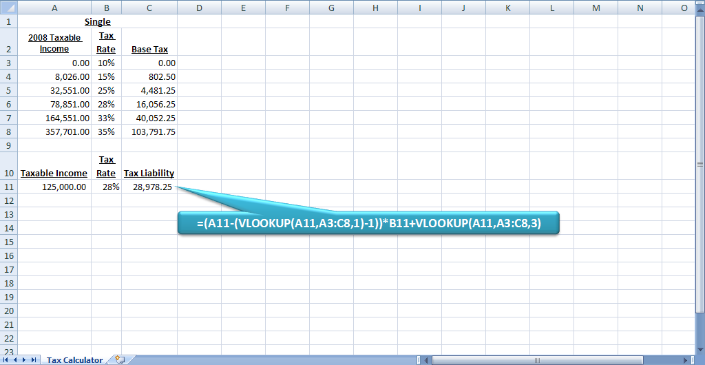 Figure 2: The spreadsheet now calculates the tax liability.
Expand the Calculator
Since our formula works with a single table, we’ll now add the three additional tables to the spreadsheet. After that we’ll then assign range names to each table, add a filing status input, and then incorporate the INDIRECT function into our VLOOKUP formulas. Here’s how:
- Add the remaining three tables, as shown in Figure 3:
|
Married-Filing Jointly |
||
|
2008 Taxable Income |
Marginal Rate |
Base Tax |
|
0.00 |
10% |
0.00 |
|
16,051.00 |
15% |
1,605.00 |
|
65,101.00 |
25% |
8,962.50 |
|
131,451.00 |
28% |
25,550.00 |
|
200,301.00 |
33% |
44,828.00 |
|
357,701.00 |
35% |
96,770.00 |
|
Married-Filing Single |
||
|
2008 Taxable Income |
Marginal Rate |
Base Tax |
|
0.00 |
10% |
0.00 |
|
8,026.00 |
15% |
802.50 |
|
32,551.00 |
25% |
4,481.25 |
|
65,726.00 |
28% |
12,775.00 |
|
100,151.00 |
33% |
22,414.00 |
|
178,851.00 |
35% |
48,385.00 |
|
Head of Household |
||
|
2008 Taxable Income |
Marginal Rate |
Base Tax |
|
0.00 |
10% |
0.00 |
|
11,451.00 |
15% |
1,145.00 |
|
43,651.00 |
25% |
5,975.00 |
|
112,651.00 |
28% |
23,225.00 |
|
182,401.00 |
33% |
42,755.00 |
|
357,701.00 |
35% |
100,605.00 |
 Figure 3: Add the additional tables to your spreadsheet.
- The next step is to assign a range name to each table. This will allow us to refer to each table by name, such as Single, rather than by cell coordinates, such as A3:C8. To do so, select cells A3:C8, and then enter the word Single in the Name Box, as shown in Figure 5.
 Figure 4: You can use the Name Box to assign a range name to a cell or block of cells.
- Select cells E3:G8, and assign the name MarriedJoint
- Select cells I3:K8, and assign the name MarriedSingle.
- Select cells M3:O8, and assign the name HeadOfHousehold.
Name limitations: You cannot use spaces or dashes within range names, nor can you start a range name with a number. Many users use the underscore character in place of spaces, such as Head_of_Household.
- Enter the words Filing Status in cell D10.
- Use the Data Validation feature to create an in-cell drop-down list in cell D11:
- Excel 2007: Choose the Data Validation icon in the Data Tools section of the Data ribbon.
Excel 2003 or earlier: Choose Tools, and then Data Validation.
- In all versions of Excel, choose List, and then enter this into the Source field, as shown in Figure 5:
Single,MarriedJoint,MarriedSingle,HOH
Caution: Be sure that the contents of the Source field exactly match the range names that you assigned to each of the tables.
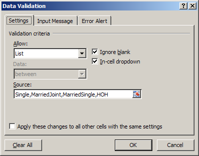
Figure 5: Enter these settings in the Data Validation window.
- Click OK. At this point, a drop-down list should appear when you click on cell D11, as shown in Figure 6.
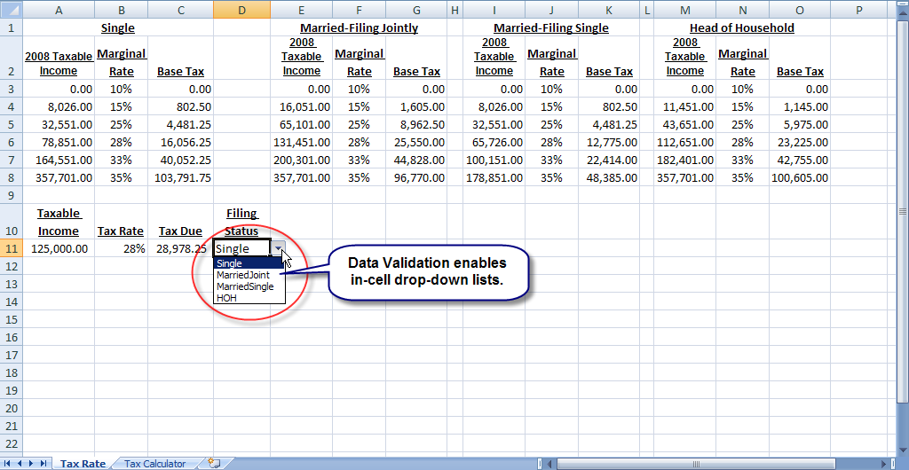
Figure 6: Data Validation provides an in-cell dropdown list.
- Modify the formula in cell B11 to use the INDIRECT function:
=VLOOKUP(A11,INDIRECT(D11),2)
Tip: You’re simply replacing A3:C8 with INDIRECT(D11).
- Modify the formula in cell C11 to use the INDIRECT function:
=(A11-(VLOOKUP(A11,INDIRECT(D11),1)-1))*B11+VLOOKUP(A11,INDIRECT(D11),3)
INDIRECT: The INDIRECT function enables you to convert text into an Excel address. In this case, we can use INDIRECT to change between one of four tables without having to modify the formulas in cells B11 and C11.
- At this point you can test your work by making different choices from the drop-down list in cell D11:
- MarriedJoint should cause cell C11 to return $23,937.50
- MarriedSingle should cause cell C11 to return $30,614.50
- HOH should cause cell C11 to return $26,683.00
You now have a functional tax calculator that we’ll streamline next month in Part 2 of this series.
The views and opinions expressed in this column are those of the author and do not necessarily reflect theopinions of Microsoft.
This article first appeared Microsoft Professional Accountant’s Network newsletter.
David H. Ringstrom, CPA heads up Accounting Advisors, Inc., an Atlanta-based software and database consulting firm providing training and consulting services nationwide. Contact David at david@acctadv.com or follow him on Twitter. David speaks at conferences about Microsoft Excel, and presents webcasts for several CPE providers, including AccountingWEB partner CPE Link
Aug 15
How to Speed Up Microsoft Excel’s Help Window
About the author:
David H. Ringstrom, CPA heads up Accounting Advisors, Inc., an Atlanta-based software and database consulting firm providing training and consulting services nationwide. Contact David at david@acctadv.com or follow him on Twitter. David speaks at conferences about Microsoft Excel, and presents webcasts for several CPE providers, including AccountingWEB partner CPE Link
Aug 08
Maximizing Excel’s Recent Items Menu
Continue reading this article where it first appeared: www.accountingweb.com
David H. Ringstrom, CPA heads up Accounting Advisors, Inc., an Atlanta-based software and database consulting firm providing training and consulting services nationwide. Contact David at david@acctadv.com or follow him on Twitter. David speaks at conferences about Microsoft Excel, and presents webcasts for several CPE providers, including AccountingWEB partner CPE Link.
Aug 02
Converting a Digital Photo into an Excel Spreadsheet
By David Ringstrom, CPA
In an unlikely mash-up, Matt Parker of Think Maths offers a free tool that converts a digital photo of your choice into an Excel spreadsheet. According to the website, “digital photographs are actually just spreadsheets. When you take a photo, your camera measures the amount of red, green, and blue light hitting each pixel, ranks them on a scale of 0 to 255, and then records those values as a spreadsheet.” Parker’s website is able to extract said values from a digital photo, record the numeric values in worksheet cells, and then use Excel’s Conditional Formatting feature to recreate the photograph.
David H. Ringstrom, CPA heads up Accounting Advisors, Inc., an Atlanta-based software and database consulting firm providing training and consulting services nationwide. Contact David at david@acctadv.com or follow him on Twitter. David speaks at conferences about Microsoft Excel, and presents webcasts for several CPE providers, including AccountingWEB partner CPE Link
Jul 26
How to Automate Text File Links in Microsoft Excel
Some time ago, I explained how to use Excel’s Text to Columns Wizard for separating text within a spreadsheet into columns. Although this approach is helpful for data that’s in a spreadsheet, in other cases, you may wish to link spreadsheets to text files that change periodically. In this article, I’ll walk you through the steps of automating this process.
Continue reading this article where it first appeared: www.accountingweb.com .
David H. Ringstrom, CPA heads up Accounting Advisors, Inc., an Atlanta-based software and database consulting firm providing training and consulting services nationwide. Contact David at david@acctadv.com or follow him on Twitter. David speaks at conferences about Microsoft Excel, and presents webcasts for several CPE providers, including AccountingWEB partner CPE Link
Jul 12
How to Eliminate a Common Spreadsheet Design Flaw
Data within Excel spreadsheets is commonly organized in columns, with explanatory titles at the top of each section. When carrying out this most basic of data entry tasks, many Excel users often unwittingly cause Excel to be harder to use. Whenever column headings within a worksheet span two or more rows, a cascade of issues can occur. Fortunately, a simple technique can help you avoid frustration and save time when working in Microsoft Excel.
Continue reading this article where it first appeared: www.accountingweb.com .
David H. Ringstrom, CPA heads up Accounting Advisors, Inc., an Atlanta-based software and database consulting firm providing training and consulting services nationwide. Contact David at david@acctadv.com or follow him on Twitter. David speaks at conferences about Microsoft Excel, and presents webcasts for several CPE providers, including AccountingWEB partner CPE Link
Jun 28
Three Ways to Convert Text-Based Numbers to Values
Periodically, you may encounter numbers in Excel that you can’t sum or use arithmetically. A common cause for this is numbers formatted as text. Often, reports exported from other programs, such as an accounting package, will be formatted as text or they might contain embedded spaces.
- Excel 2007 and later or Excel:Mac 2011: Determine if the word Text appears on the Home tab, as shown in Figure 1.
- Excel 2003 and earlier: Choose Format, Cells, and then determine if the Number tab is set to Text.


David H. Ringstrom, CPA heads up Accounting Advisors, Inc., an Atlanta-based software and database consulting firm providing training and consulting services nationwide. Contact David at david@acctadv.com or follow him on Twitter. David speaks at conferences about Microsoft Excel, and presents webcasts for several CPE providers, including AccountingWEB partner CPE Link
Jun 24
Automating Data Validation Lists in Excel
By David Ringstrom, CPA
- Excel 2007 and later – Choose Insert and then Table. Make sure that My Table Has Headers is selected and then click OK.
- Excel:Mac 2011 – On the Tables tab of the ribbon, click the arrow next to the New command and then choose Insert Table with Headers.
- Excel 2003 and earlier – Choose Data, List, and then Create List.

- Excel 2007 and later – On the Formulas tab choose Define Name.
- Excel 2003 and earlier, or Excel – Mac 2011: Choose Insert, Name, and then Define.

 [1]
[1]


David H. Ringstrom, CPA heads up Accounting Advisors, Inc., an Atlanta-based software and database consulting firm providing training and consulting services nationwide. Contact David at david@acctadv.com or follow him on Twitter. David speaks at conferences about Microsoft Excel, and presents webcasts for several CPE providers, including AccountingWEB partner CPE Link
Jun 14
Improving the Integrity of Excel’s SUM Function
By David Ringstrom, CPA
My unscientific observation is that the SUM function is the most widely used function within Excel spreadsheets. This function makes it easy to add up multiple cells at once without laboriously adding multiple cells together individually.
- Click once on cell A1 and then press Ctrl-A. This will select the contiguous area, which we need to expand by one row and one column.
- Hold down the Shift key, then tap the Down arrow, and then the Right arrow. At this point, your selection should look like Step 1 of Figure 1.
- Press Alt-Equal Sign in Windows, or on a Mac, press Command-Shift-T. Alternatively, you can click the AutoSum icon, which looks like a Greek E. Any of these actions should add totals to row 4 and column H simultaneously. Do be sure to select the cells you wish to sum; otherwise, AutoSum will place a SUM function in the first numeric cell within the current region of your spreadsheet.

Figure 1: You can use AutoSum to add totals to the row below and column to the right if you expand the initial selection.
- Insert a new row at row 4 so that the totals move down to row 5. Label cell A4 as Pears, and then enter 1000 in cells B4 through G4.
- Notice how the totals in row 5 don’t reflect the additional amount that was added for each month.

Figure 2: The totals don’t reflect the additional amount that has been added for each month.
- Insert a blank row just above the total row, which in this case now appears on row 5. Change the row height to half of its normal height. An easy way to do so is to click on the row number on the worksheet frame and then drag the bottom of the row upward slightly. Next, adjust the SUM formulas in row 6 to be: =SUM(B1:B5).

Figure 3: Insert a blank row just above the total row to avoid adjusting the SUM formula each time a new item is added.
David H. Ringstrom, CPA heads up Accounting Advisors, Inc., an Atlanta-based software and database consulting firm providing training and consulting services nationwide. Contact David at david@acctadv.com or follow him on Twitter. David speaks at conferences about Microsoft Excel, and presents webcasts for several CPE providers, including AccountingWEB partner CPE Link
Jun 09
Microsoft’s Chip In Program Offers Crowdfunded Laptops to Students
Microsoft is dipping its corporate toe into the crowdfunding pool. An experimental program dubbedChip In allows students to tap friends and relatives in a quest to fund their next computer. The program will run through September 1, 2013, and offers a 10 percent discount on a selection of name-brand laptops, tablets, and all-in-one computers. Fleet-footed student funders can also score a free, four-year subscription to Office 365 University.
David H. Ringstrom, CPA heads up Accounting Advisors, Inc., an Atlanta-based software and database consulting firm providing training and consulting services nationwide. Contact David at david@acctadv.com or follow him on Twitter. David speaks at conferences about Microsoft Excel, and presents webcasts for several CPE providers, including AccountingWEB partner CPE Link
Jun 04
Resolving #VALUE! Errors in Microsoft Excel
By David Ringstrom, CPA
It’s a frustrating experience when a simple Excel spreadsheet displays #VALUE! in a worksheet cell rather than the expected result. Many times the problem is obvious, in that you’ve tried to do arithmetic using text and numbers, but sometimes the culprit is harder to track down.


- Select one or more cells in a single column, choose Text to Columns from the Data tab or menu, and then click Finish.
- Enter the number 1 in a blank worksheet cell and then copy it to the clipboard.
- Select the range of cells you wish to convert to values and then right-click and choose Paste Special.
- Double-click on Multiply.
David H. Ringstrom, CPA heads up Accounting Advisors, Inc., an Atlanta-based software and database consulting firm providing training and consulting services nationwide. Contact David at david@acctadv.com or follow him on Twitter. David speaks at conferences about Microsoft Excel, and presents webcasts for several CPE providers, including AccountingWEB partner CPE Link
May 29
Overcome a Nuance of Excel’s Subtotal Feature
By David Ringstrom, CPA
Many users rely on the Subtotal feature in Excel to instantly insert totals, averages, counts, or other statistics into a list. As you’ll see, the feature is easy to use – until you want to copy or format just the total rows. In this article, I’ll explain the nuance so that you’ll be in complete control of this feature.
- Select any cell within your list.
- Choose the Subtotal command on the Data tab in Excel 2007 and later, or the Data menu in Excel 2003 and earlier.
- Select the Cases Sold field, and then click OK.


- As shown in Figure 5, select the cells that you wish to copy or format.
- Press Ctrl-G to display the Go To dialog box and then click the Special button.
- Double-click Visible Cells Only.

- In any version of Excel, press F5 instead of Ctrl-G.
- In Excel 2007 and later, choose the Find & Select command on the Home Tab and then choose Go To Special.
- In Excel 2003 and earlier, choose Edit, Go To, and then click the Special button.
David H. Ringstrom, CPA heads up Accounting Advisors, Inc., an Atlanta-based software and database consulting firm providing training and consulting services nationwide. Contact David at david@acctadv.com or follow him on Twitter. David speaks at conferences about Microsoft Excel, and presents webcasts for several CPE providers, including AccountingWEB partner CPE Link
May 17
Farewell, Lotus 1-2-3
By David Ringstrom, CPA
IBM recently announced that Lotus 1-2-3 will no longer be available for purchase. Most readers of this article will likely have one of two reactions: “What is Lotus 1-2-3?” or else an incredulous “Lotus 1-2-3 was still on the market?” If you’re of a certain age, you may wistfully remember Lotus 1-2-3 as your first spreadsheet program.
David H. Ringstrom, CPA heads up Accounting Advisors, Inc., an Atlanta-based software and database consulting firm providing training and consulting services nationwide. Contact David at david@acctadv.com or follow him on Twitter. David speaks at conferences about Microsoft Excel, and presents webcasts for several CPE providers, including AccountingWEB partner CPE Link
